Sometime near the end of last year, I came across a blog post by Scott Alexander giving an overview of Anthropic’s recent work on language model interpretability. The post is entitled “God Help Us, Let's Try To Understand AI Monosemanticity” which is highly provocative and slightly alarming, especially given the wild acceleration that AI capabilities research has experienced as of late. Scott wants God’s help both because Anthropic’s research is kind of dense and seemingly unapproachable at first glance, and also because of the apparent dire need to understand what these models are actually doing. After reading through Scott’s post and Anthropic’s publication, however, I became less alarmed and more excited — the core of the research is actually pretty straightforward, but the findings are fascinating. If you’re not familiar with the research, I’d highly recommend reading Scott’s post, but here’s the gist:
Large language models like ChatGPT (or Anthropic’s Claude, or Google’s Gemini) are extremely powerful and clearly employ some kind of complex, learned logic which we’d like to understand. One way to do this is to look at the atomic components of these models, called artificial neurons, and try to discern a function for each one. If we do this naively, however, we find that single neurons actually tend to correspond to multiple functions— this is called “superposition”. For example, the authors find a single neuron which “responds to a mixture of academic citations, English dialogue, HTTP requests, and Korean text”. This is what they call “polysemanticity”, and makes interpreting the model almost impossible. The researchers propose a technique using sparse dictionary learning which decomposes these neurons into “features” — linear combinations of neurons which together exhibit “monosemanticity” — which are individually interpretable (and thus allow a first look into how these models are working).
I found these findings particularly fascinating for two reasons:
To me, this is the first really compelling breakthrough in LLM interpretability. It feels like a zero-to-one moment for the field, and represents new velocity in an area that is currently way, way behind AI capabilities research.
Reading through the paper, I was pretty sure I could reproduce the core findings on my MacBook Pro, from scratch!
This post details my journey in doing so, and also attempts to give clear explanations of the technical details of Anthropic’s work. You may also be interested in the GitHub repository.
If you’re reading this you probably already have some idea of how neural networks work, but let’s quickly go over the general concepts anyway. To a computer, a language model is a bunch of matrices to multiply and add together in a specific way. Humans have a more abstract conceptual model of how they work, and we generally describe them as networks made up of artificial neurons. They kind of look like this:

The two vertical columns of black circles are called “layers”, and, as the input signal travels through the network from left to right, these layers have “activations” which can be represented as vectors. These activation vectors sort of represent what the model is “thinking” given some input, and contain the neurons that we want to interpret.
In “Toy Models of Superposition”, Anthropic researchers find that it is rarely possible to assign a single semantic meaning to any given neuron, even in very small models. Instead, groups of neurons can encode many different, completely unrelated features. Importantly, the number of distinct features encoded by a set of neurons is usually greater than the number of neurons in the set; neuron sets form low-dimensional subspaces which each encode more features than there are neurons in the set1. Thus, the problem becomes finding which sets of neurons encode which sets of features, and what linear combinations of neurons within these sets correspond to which individual features.
There’s another framing of this problem which I think is important to understand: What we have is a dense model, where lots of neurons fire at the same time, and any given neuron may fire under a variety of circumstances. What we want a model which is sparse, where only a small number of features are active at once. This way, we can clearly observe which stimuli cause which features to be active, and which features correspond with different behaviors in the model.
Anthropic thought of a whole bunch of techniques to create this sparse model, and found one that worked well: sparse dictionary learning.
Modern language models overwhelmingly use some variant of the transformer architecture. It’s not necessary to go into the details of how it works in this post2, but here’s a rough approximation:
In the context of language models, a transformer takes as input a string of text encoded as tokens, and outputs probabilities for each potential next token. A transformer is made up of some number of transformer blocks, followed by a fully-connected layer at the very end. Usually, transformers have lots of transformer blocks one after another, but the network used in this research only has one for simplicity (the authors call it “the simplest language model we profoundly don't understand”). Inside a transformer block, you have self-attention heads followed by something called a multi-layer perceptron (MLP). You might choose to think about the function of these two components like this: the attention heads tell the model which parts of the input to think about, and the MLP does the thinking. The MLP is itself a very simple feed-forward neural network with only an input (the output of the attention heads), a hidden layer, and an output.
This hidden layer is the one we’re interested in, and we will largely ignore the rest of the model. Every time we run some input (a string of text) through the transformer, we can pull out activations of this layer as a vectors. Moving forward, I’ll be referring to these vectors as “MLP activation vectors” or simply “activation vectors”.
I trained an implementation of this one-layer transformer on a subset of the Pile3, and the output looks something like this:
★.Fallings motorcycle ozPhoto(
at a fat of version of “I get along that my wife’s next week—rail," MiddlemondBlue said.
United States Courses (UK)
Mark Ackermanishing) is reflected in the country, the Commander
Demos. at the Mancalysis, Robert Duffy has developed an appreciation of the Interior Cance below, incomplete, and the world contains many misconceptions to open, and possibly a comparison of an area.
Smooth War does not have created at least, in people must know which he is physical and will seem
It’s mostly gibberish — the model used by the researchers is simply not large enough to produce anything meaningful — but the output nonetheless contains mostly correct grammatical structures and punctuation. There’s enough structure that we should be able to extract meaningful features.
To get an idea of how these neurons behave, we can take a look at the neuron density histogram for our model:

This histogram gives us an idea of how often neurons are firing on inputs from our dataset. It was generated by randomly sampling a large number of inputs and looking at the activations for each neuron in the MLP activation vector. If a neuron’s activation is nonzero, it is considered to be firing. We record the proportion of tokens across all our inputs for which each neuron fires and plot these values in a histogram.
We can see that almost all of the neurons fire more than 10% of the time, and around half fire more than 25% of the time. This is bad for interpretability, since it means that most of our neurons are firing either for very broad concepts or for multiple different concepts, otherwise we’d observe them firing less frequently. In order for neurons to be interpretable, we’d like them to fire for singular, distinct, and narrow concepts, which means that their activations need to be infrequent; the activation vector needs to be sparse.
How can we make these activations sparse? The authors employ the use of something called a sparse autoencoder. This is an auxiliary network, trained separately from the transformer. The autoencoder takes the MLP activation vector as input, encodes it into an intermediate representation, and then tries to reconstruct it again from this new representation. If we force the intermediate representation to be sparse, we can try to use this representation to interpret the MLP activations.
Warning: This part of the post is extremely technical— I won’t be offended if you skip to the results.
Our sparse autoencoder has a single hidden layer. The input and output of the autoencoder have the same shape as the activation vector we want to transform, while the shape of the middle layer corresponds with the number of features we are targeting. I chose to use an autoencoder with 1024 features, which is large enough to have more features than input neurons, but small enough to train quickly. These features are those which we want to be able to interpret, and in order to ensure that they are monosemantic, we need to enforce that they have sparse activation. We do this by computing the L1 norm of the activations of this layer during training, scaling it, and adding it to our loss function (the rest of the loss function is standard mean squared error). The L1 norm is just the sum of absolute values for each feature activation; my intuition is that this works because it applies even negative pressure to all activations, while the mean squared error component of the loss applies positive, quadratic pressure to high signal activations. It’s a balancing act, and because small activations are more likely to be noise rather than signal, they get pushed down to zero.
What we have so far is a sparse autoencoder with an L1 penalty on feature activations. The authors take this a step further and implements a statistical method called sparse dictionary learning into the training loop. We’ll implement this too, here’s how it works:
In our training loop, we explicitly enforce that each row of the decoder’s weight matrix has unit L2 norm and mean zero. If you think about it, this means that every element of the autoencoder’s hidden layer corresponds to a different direction in vector space. This is the “dictionary” in sparse dictionary learning; every element in the dictionary is a direction with the same magnitude. Because the output of the autoencoder is a reconstruction of the original MLP activation vector, we are representing the MLP activation vector as a linear combination of a small number of these dictionary entries. The activations of the autoencoder’s hidden layer are the coefficients of the elements in this linear combination.
Let’s take a look at the equations Anthropic provides describing the forward pass and loss function to further elucidate this training mechanism:
\(f = \text{ReLU}(W_e\bar{x} + b_e)\)
\(\mathcal{L} = \frac{1}{|X|} \sum_{x \in X} \left\| x - \hat{x} \right\|^2 + \lambda \|f\|_1\)
Here, x is out input (the MLP activation vector). We, Wd are the weights of our encoder and decoder and be, bd are the biases. Curiously, the first step is to subtract the decoder bias from the input, before running a forward pass through the encoder. Adding the decoder bias back in is also the last step in the forward pass; these two steps allow our model to “center” the input before encoding and decoding. Recall that we are normalizing our decoder weights to have row-wise zero mean — this means that it’s favorable for the input vectors to also have zero mean on average, so this centering allows our autoencoder to learn more efficient sparse representations.
The rest of the forward pass (apply encoder weights + bias, ReLU, apply decoder weights + bias) is standard. Also note the last term of the last equation — this is the L1 norm of f, our encoded representation. Adding this to the loss function encourages the autoencoder to learn sparse representations. Lambda is a hyperparameter which we can tune to increase or decrease the sparsity of these representations.
It’s not described in the above equations, but we also normalize decoder weights as the last step in our training loop to enforce that each element of our dictionary has the same magnitude.
Here’s my (abridged for clarity) implementation of the autoencoder:
class SparseAutoencoder(nn.Module):
    def __init__(self, n_features, n_embed):
        super().__init__()
        self.encoder = nn.Linear(n_embed * 4, n_features)
        self.decoder = nn.Linear(n_features, n_embed * 4)
        self.relu = nn.ReLU()
    def encode(self, x_in):
        x = x_in - self.decoder.bias
        f = self.relu(self.encoder(x))
        return f
    def forward(self, x_in, compute_loss=False):
        f = self.encode(x_in)
        x = self.decoder(f)
        if compute_loss:
            recon_loss = F.mse_loss(x, x_in)
            reg_loss = f.abs().sum(dim=-1).mean()
        else:
            recon_loss = None
            reg_loss = None
        return x, recon_loss, reg_loss
    def normalize_decoder_weights(self):
        with torch.no_grad():
            self.decoder.weight.data = nn.functional.normalize(self.decoder.weight.data, p=2, dim=1)
The encode function explicitly subtracts the decoder bias before applying the encoder and ReLU. forward applies the decoder, and computes reconstruction loss and regularization loss separately. normalize_decoder_weights does what it says on the tin, and normalizes the weights of the decoder to have unit norm and zero mean.
Lastly, let’s also take a look at the code for the training loop. Anthropic has a lot of computational resources, so they first create a dataset of MLP activation vectors by running a large chunk of The Pile through the transformer and saving the activations to disk4. These vectors actually take up a huge amount of space (a token takes up four bytes, while 512 element FP16 activation vector representing this token in context is 1024 bytes), and would end up being way more storage that I have access to, so I compute them batch-by-batch in memory as part of the autoencoder’s training loop. Here’s a simplified version of my implementation:
for _ in range(num_training_steps):
    xb, _ = next(batch_iterator)  # get a batch of inputs for the transformer
    with torch.no_grad():
        x_embedding, _ = model.forward_embedding(xb)  # get MLP activation vectors for the input batch
    optimizer.zero_grad()
    outputs, recon_loss, reg_loss = autoencoder(x_embedding, compute_loss=True)
    reg_loss = lambda_reg * reg_loss
    loss = recon_loss + reg_loss  # total loss is reconstruction loss + regularization penalties
    loss.backward()
    optimizer.step()
    autoencoder.normalize_decoder_weights()  # normalize decoder weights at the end of every training step
Note the presence of normalize_decoder_weights at the end of the loop.
That’s it, pretty much. Assuming we start with a trained transformer, we can run this training loop and train our autoencoder to create sparse representations of the transformer’s MLP activations. Then, we can run something like this on a new tokenized input:
features = autoencoder.encode(transformer.forward_embedding(tokens))Now, features will contain a sparse representation of our tokenized text. If everything went well, the elements of features should be monosemantic, and interpretable!
We’ve trained an autoencoder that gives us a representation of our MLP activation vector. How do we know that this autoencoder isn’t throwing out too much information? Even if our discovered features are monosemantic, they won’t be very useful if they do not capture the majority of the transformer’s behavior. Anthropic tests this by comparing the overall loss of the original transformer (calculated on it’s training set) to the loss of the transformer if we replace the MLP activations with the autoencoder’s output5. This comparison is tricky because we only want to compare the proportion of the transformer’s loss which is caused by the MLP. In other words: The MLP component of the transformer reduces its overall loss by some amount; how much of this reduction is recovered by the autoencoder?
We can easily calculate the loss reduction contributed by the MLP by setting its activation to all-zeros6, and we can calculate the loss using the autoencoder by replacing the MLP activation with the autoencoder’s approximation. The loss ratio we’re after is given by the following equation:
\(Loss Ratio=\frac{L_{zero-ablated}-L_{approximation}}{L_{zero-ablated}-L_{original}}\)
Here, Loss Ratio represents the amount of loss reduction which is recovered by the autoencoder compared with the original transformer MLP. A value of 100% means the autoencoder captures all relevant information from the MLP, 0% means none of the information from the MLP makes it through. The loss ratio using my trained models is about 68%, while Anthropic published a value of 79% for a larger autoencoder which they trained. I think there are a couple reasons for this discrepancy: first, my model is smaller (it’s only 25% as large as the one the authors used to achieve their 79% loss ratio), which gives it less capacity to model the MLP activations. Additionally, I think it’s probably undertrained compared to Anthropic’s, and I skipped some potentially important optimizations which I’ll discuss later. Still, by this metric we’re getting around 86% of the performance that the authors achieved, which is strong enough to move forward.
It’s also important to check that the features we’re left with are actually sparse. To do that, we can compare the density histograms between MLP activations and the autoencoder’s feature activations. These histograms show how often features/neurons fire on a representative sample of inputs.

The autoencoder’s features, shown in red, are much less likely to activate than the blue transformer neurons. This is a log plot, so each tick going leftwards represents a 90% decrease in activation likelihood. You’ll notice there are still a large number of features that fire more than 10% of the time — this is not desirable, and is a consequence of the tradeoff between increasing sparsity and avoiding dead features. The big spike on the left represents a cluster of features that all activate very infrequently; the authors find something similar and call it the “ultra-low density cluster” — more on this later.
Now we can finally generate a bunch of feature vectors on new inputs, and check to see if our features are really interpretable (this is the fun part). You can skip to that analysis here**(link to results), but first I’d like to go over some additional techniques which Anthropic used to improve their feature representations which I elected not to implement.
Update: I ended up implementing the resampling technique described below after writing this post, and it considerably improved the performance of the SAE. I’ll probably write a follow-up post with more details, but for now the code is on GitHub.
There are at least two additional techniques implemented by the researchers to improve results, which I left out. I mostly did this to save time and reduce complexity; the literature suggests that these optimizations offer only marginal improvement, and they seemed difficult to debug. Looking back, I think that the first neglected optimization, neuron resampling, actually would have had a larger effect than I anticipated; this is something I’d like to investigate more in the future. Here’s how that works:
Recall that we apply a penalty to the absolute value of feature activations during training of the sparse autoencoder. Because of this, some features are killed off by the optimizer before they are able to learn anything meaningful. When this happens, it’s almost impossible for these “dead” features to learn to fire again, since their weights will be very close to zero and thus the gradient for these features will be extremely weak. To improve the learning capacity of our autoencoder, we can reinitialize the weights of these features manually to try to resuscitate them. The authors do this in a clever way:
First, check which features haven’t fired in a long time. Let D be this set of features.
Then, calculate the model’s loss on a random set of inputs I.
For each dead feature d in D, sample an input i from I by weighting each input using it’s squared loss value from the previous step.
Set the decoder weights for d to be equal to normalized i7.
Do something similar for the encoder weights8, and reset the optimizer’s parameters for d.
Based on the number of dead features I ended up with, I think implementing the above technique would be the best starting point for improving my overall results.
This brings us to the the other optimization which I left out, which is pretty straight forward:
In our training loop, we renormalize decoder weights to have unit norm. This renormalization should represent a fairly small change, but we never actually tell the optimizer about it; based on it’s gradient, the optimizer thinks it can make changes to the magnitudes of dictionary vectors. The authors remove all gradient information parallel to these vectors and find “a small but real reduction in total loss”9.
Alright, it’s time for my favorite part: exploring the extracted features. If you want, you can browse all of them here. Note: my feature browser (a markdown file on GitHub) is considerably less sophisticated than Anthropic’s.
If you really like counting, you’ll have noticed that there are a total of 576 extracted features, which is fewer than the number of neurons in our autoencoder’s hidden layer. What gives? The researchers describe an “ultralow density cluster” of features which activate extremely infrequently. Activation of these features appears to be spurious10, and it’s difficult to discern any semantic meaning for the vast majority of them. Like the researchers, I also encountered a set of features which were very unlikely to activate (I additionally observed that these features had very low activation magnitudes when they did activate). In the feature density histogram above, these features are contained in the far-left spike, around 0.001% activation density. I chose to leave these features out of my analysis since they appear to be very low-signal and make things a lot messier if they’re left in. Because they activate so infrequently and with such small magnitudes, they should only have a very small contribution to overall loss11, so I believe ignoring them is OK to do from a statistical rigor perspective. On the other hand, it’s worth noting that the researchers’ ultralow density clusters for their models tend to be smaller and even less dense than what I found. This is very likely a consequence of the low-density neuron resampling they did during training, which I’ve described above. I left this out, which I think caused me to end up with a much higher proportion of low-density features. Anyway, I filtered out all features which fire on fewer than 1 in 10,000 tokens, which leaves a bit more than half. This still yields a greater number of features than input neurons from the transformer MLP, which is something I wanted to achieve.
With that out of the way let’s look at a few features that I find most interesting. These are cherry-picked, so not exactly representative of the full set, but fun to look at nonetheless. We’ll go over a more quantitative analysis further down.

215: This feature appears to fire on suffixes in Spanish, French, and Portuguese language contexts. I find it fascinating that this feature fires specifically on suffixes in these languages, instead of any context written in one of these languages.

171: This feature fires for alphanumeric strings, usually hexadecimal or base 64.

120: This feature indicates the presence of a modal verb, such as “could”, “might”, or “must”.
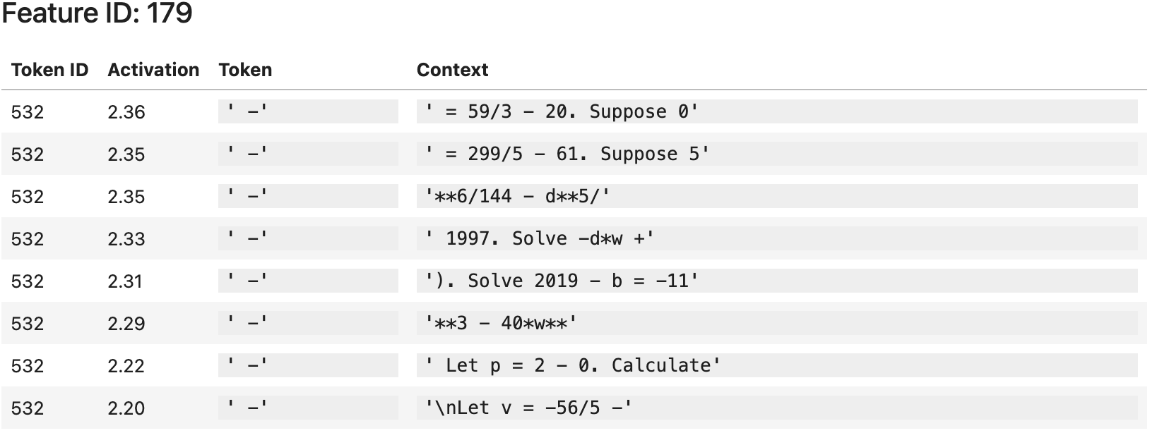
179: Seems to only fire for hyphens, always in the context of subtraction or negation.

157: Fires for various tokens in the context of cell and molecular biology.
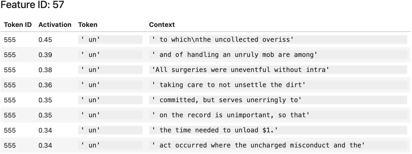
57: The “un” prefix.

229: Tokens that are a part of inline LaTeX expressions (denoted by opening and closing dollar signs).

211: Closing parenthesis in mathematical function declarations using the word “Let”.
Let’s also look at a sample of results that gives us a more representative view of the entire set. Here’s an overview of each of the first 8 features in the filtered feature set12:
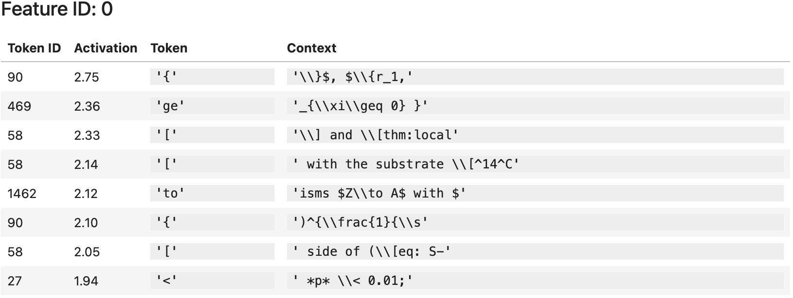
0: This feature appears to fire for various tokens which are part a LaTeX expression. It seems to fire most often for open brackets.

2: This one is not as obvious, but the contexts do have some vague similarity if you squint. I think it could be characterized somewhere along the lines of “persuasive arguments” or “decision making”. Maybe looking at longer contexts would help, or maybe this feature is just not very interpretable; some of my autoencoder’s features remain difficult to interpret.

3: Fires for commas in various contexts.

5: This feature fires in mathematical contexts. It looks like it fires specifically in instructional contexts, like proofs or exam questions.

6: Fires for the word “the” in various contexts.
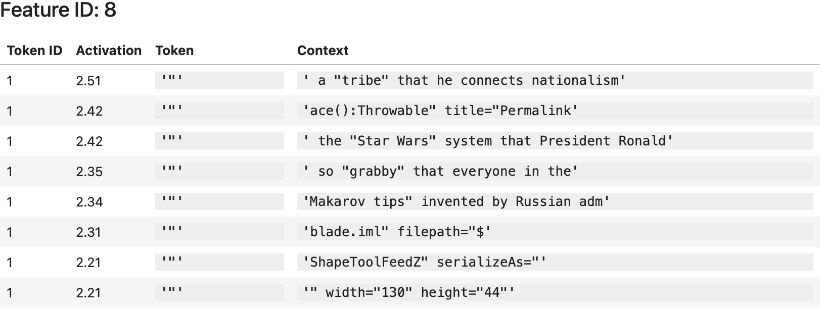
8: Fires for closing quotation marks.

9: This one is also tricky, but it looks like this feature tends to fire on directional, qualitative judgements: “less valuable”, “better”, “perfect”, “good”, “really sad”, etc. “Social” is an outlier, though.
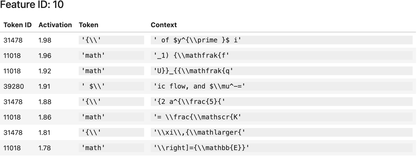
10: Like the first feature, this feature also fires for various LaTeX contexts.
It’s fun to look at the extracted features, but are they really more interpretable than the transformer neurons that we started with? I decided to do a blind test where I randomly sample from transformer neurons and autoencoder features, and rate the subjective interpretability on a 1 through 5 scale (1 is seemingly random activation, 5 is clearly interpretable and monosemantic). The resulting scores are displayed in the left histogram in the figure below.
The results look very good, with a huge peak at 5 for extracted features, and 1 for transformer neurons — the features appear to be highly interpretable and monosemantic! The graph actually looks a little too-good-to-be-true to me, and I fear that I introduced some bias by personally looking at so many feature activation contexts and subconsciously learning how to distinguish them from transformer neurons, independent of how interpretable they are. I decided to run an additional study using the same methodology, but with GPT-4 as the subject instead of myself. I made sure not to include any examples in the prompt to minimize bias, and described only a principles-based evaluation criteria. The resulting histogram (on right side of the figure below) is much less spiky, but still shows GPT-4 preferring autoencoder features over transformer neurons when scoring interpretability.

Scoring the interpretability of features is somewhat subjective, but if there is some “true” scoring, I believe it would be somewhere in the middle of these two graphs. Anthropic did a similar analysis, albeit with more rigor13, which resulted in the following figures:

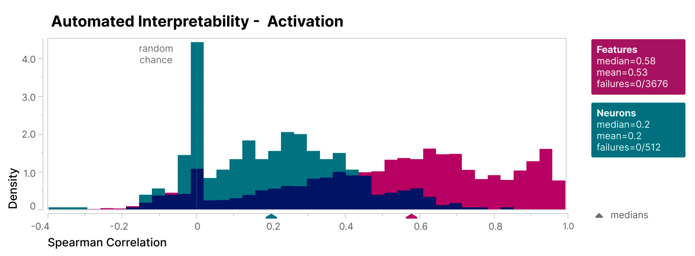
Theirs look a lot like mine! At least to my eyes — you can judge for yourself.
I had a lot of fun with this research, it really does feel like you’re digging into the internal circuitry of a transformer and finding out what makes it tick. There’s definitely a lot of work that needs to be done to scale this for use in any of the LLMs in use today, but I like how Anthropic puts it: “For the first time, we feel that the next primary obstacle to interpreting large language models is engineering rather than science”.